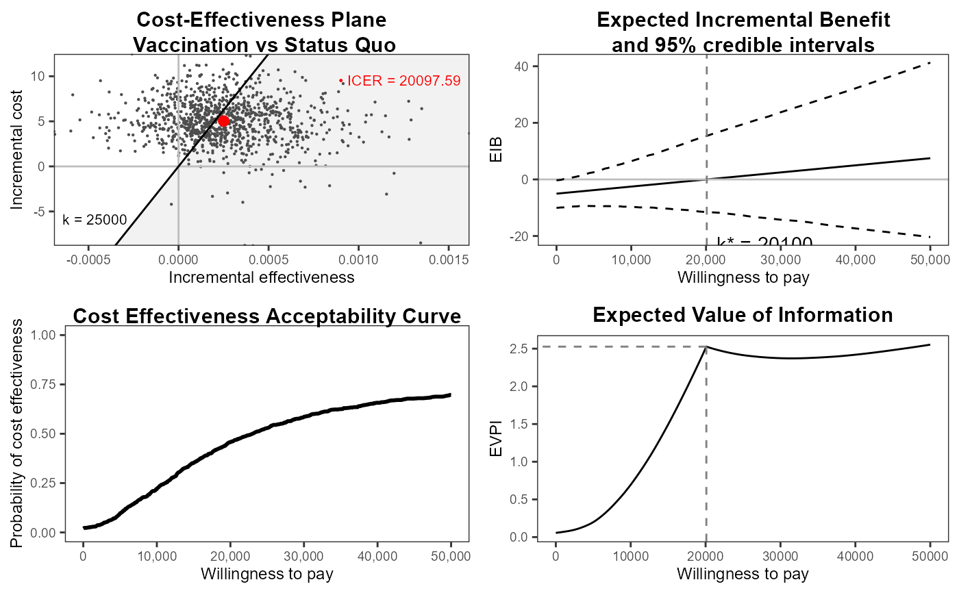
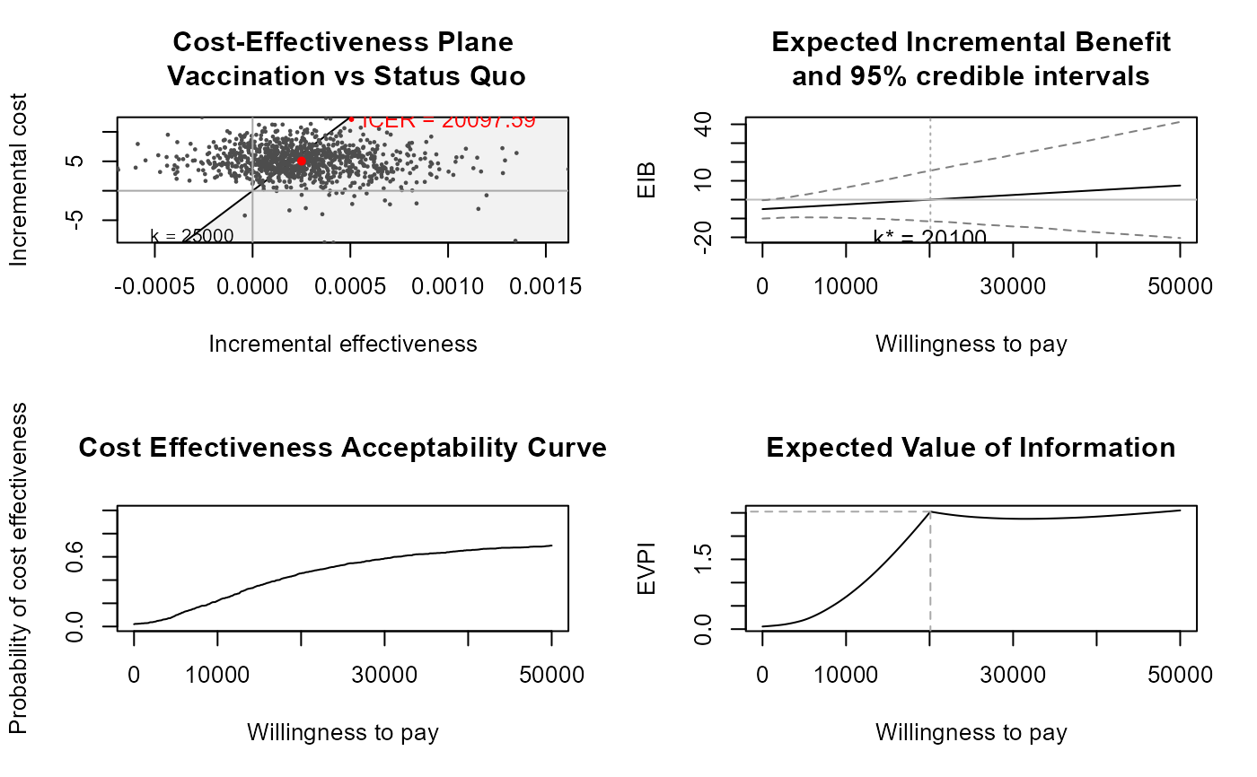
Summary Plot of the Health Economic Analysis

Plots in a single graph the Cost-Effectiveness plane, the Expected Incremental Benefit, the CEAC and the EVPI.

Usage

# S3 method for bcea
plot(
  x,
  comparison = NULL,
  wtp = 25000,
  pos = FALSE,
  graph = c("base", "ggplot2"),
  ...
)

Arguments

x: A bcea object containing the results of the Bayesian modelling and the economic evaluation.
comparison: Selects the comparator, in case of more than two interventions being analysed. Default as NULL plots all the comparisons together. Any subset of the possible comparisons can be selected (e.g., comparison=c(1,3) or comparison=2).
wtp: The value of the willingness to pay parameter. It is passed to ceplane.plot().
pos: Parameter to set the position of the legend (only relevant for multiple interventions, ie more than 2 interventions being compared). Can be given in form of a string (bottom|top)(right|left) for base graphics and bottom|top|left|right for ggplot2. It can be a two-elements vector, which specifies the relative position on the x and y axis respectively, or alternatively it can be in form of a logical variable, with FALSE indicating to use the default position and TRUE to place it on the bottom of the plot.
graph: A string used to select the graphical engine to use for plotting. Should (partial-)match the two options "base" or "ggplot2". Default value is "base".
...: Arguments to be passed to the methods ceplane.plot() and eib.plot(). Please see the manual pages for the individual functions. Arguments like size, ICER.size and plot.cri can be supplied to the functions in this way. In addition if graph="ggplot2" and the arguments are named theme objects they will be added to each plot.

Value

A plot with four graphical summaries of the health economic evaluation.

Details

The default position of the legend for the cost-effectiveness plane (produced by ceplane.plot()) is set to c(1, 1.025) overriding its default for pos=FALSE, since multiple ggplot2 plots are rendered in a slightly different way than single plots.

References

Baio G, Dawid aP (2011). “Probabilistic sensitivity analysis in health economics.” Stat. Methods Med. Res., 1--20. ISSN 1477-0334, doi:10.1177/0962280211419832 , https://pubmed.ncbi.nlm.nih.gov/21930515/.

Baio G (2013). Bayesian Methods in Health Economics. CRC.

Author

Gianluca Baio, Andrea Berardi

Examples

# See Baio G., Dawid A.P. (2011) for a detailed description of the 
# Bayesian model and economic problem

# Load the processed results of the MCMC simulation model
data(Vaccine)

# Runs the health economic evaluation using BCEA
he <- bcea(
       e=eff, c=cost,        # defines the variables of 
                             #  effectiveness and cost
       ref=2,                # selects the 2nd row of (e,c) 
                             #  as containing the reference intervention
       interventions=treats, # defines the labels to be associated 
                             #  with each intervention
       Kmax=50000,           # maximum value possible for the willingness 
                             #  to pay threshold; implies that k is chosen 
                             #  in a grid from the interval (0,Kmax)
       plot=FALSE            # does not produce graphical outputs
      )

# Plots the summary plots for the "bcea" object m using base graphics
plot(he, graph = "base")


# Plots the same summary plots using ggplot2
if(require(ggplot2)){
plot(he, graph = "ggplot2")

##### Example of a customized plot.bcea with ggplot2
plot(he,
  graph = "ggplot2",                                      # use ggplot2
  theme = theme(plot.title=element_text(size=rel(1.25))), # theme elements must have a name
  ICER_size = 1.5,                                        # hidden option in ceplane.plot
  size = rel(2.5)                                         # modifies the size of k = labels
  )                                                       # in ceplane.plot and eib.plot
}