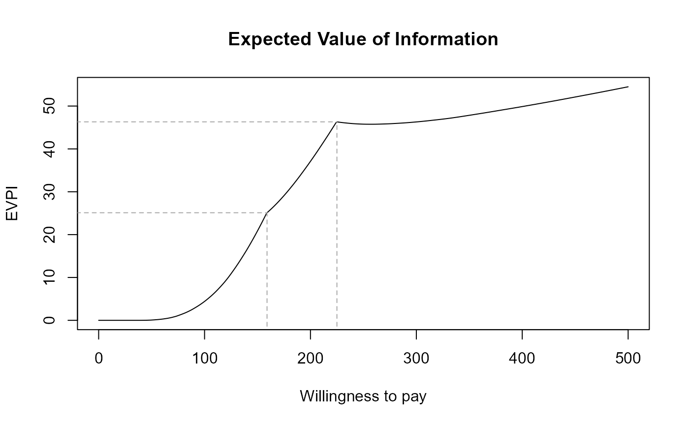
Plots the Expected Value of Information (EVI) against the willingness to pay.
Usage
# S3 method for bcea
evi.plot(he, graph = c("base", "ggplot2", "plotly"), ...)

evi.plot(he, ...)
Arguments
- he
A
bceaobject containing the results of the Bayesian modelling and the economic evaluation.- graph
A string used to select the graphical engine to use for plotting. Should (partial-)match the three options
"base","ggplot2"or"plotly". Default value is"base".- ...
Additional graphical arguments:
line_colorsto specify the EVPI line colour - all graph types.line_typesto specify the line type (lty) - all graph types.area_includeto specify whether to include the area under the EVPI curve - plotly only.area_colorto specify the area under the colour curve - plotly only.
Value
- eib
If
graph="ggplot2"a ggplot object, or ifgraph="plotly"a plotly object containing the requested plot. Nothing is returned whengraph="base", the default.
The function produces a plot of the Expected Value of Information as a function of the discrete grid approximation of the willingness to pay parameter. The break even point(s) (i.e. the point in which the EIB=0, ie when the optimal decision changes from one intervention to another) is(are) also showed.
References
Baio G, Dawid aP (2011). “Probabilistic sensitivity analysis in health economics.” Stat. Methods Med. Res., 1--20. ISSN 1477-0334, doi:10.1177/0962280211419832 , https://pubmed.ncbi.nlm.nih.gov/21930515/.
Baio G (2013). Bayesian Methods in Health Economics. CRC.
Examples
data(Vaccine)
m <- bcea(
      e=eff,
      c=cost,               # defines the variables of
                            #  effectiveness and cost
      ref=2,                # selects the 2nd row of (e, c)
                            #  as containing the reference intervention
      interventions=treats, # defines the labels to be associated
                            #  with each intervention
      Kmax=50000,           # maximum value possible for the willingness
                            #  to pay threshold; implies that k is chosen
                            #  in a grid from the interval (0, Kmax)
      plot=FALSE            # plots the results
)
evi.plot(m)


data(Smoking)
treats <- c("No intervention", "Self-help",
            "Individual counselling", "Group counselling")
m <- bcea(eff, cost, ref = 4, interventions = treats, Kmax = 500)
evi.plot(m)

