Getting Started • BCEA

This vignette will demonstrate a simple cost-effectiveness analysis using BCEA using the smoking cessation data set contained in the package.

library(BCEA)

Load the data.

data(Smoking)

This study has four interventions.

treats <- c("No intervention", "Self-help", "Individual counselling", "Group counselling")

Setting the reference group (ref) to Group counselling and the maximum willingness to pay (Kmax) as 500.

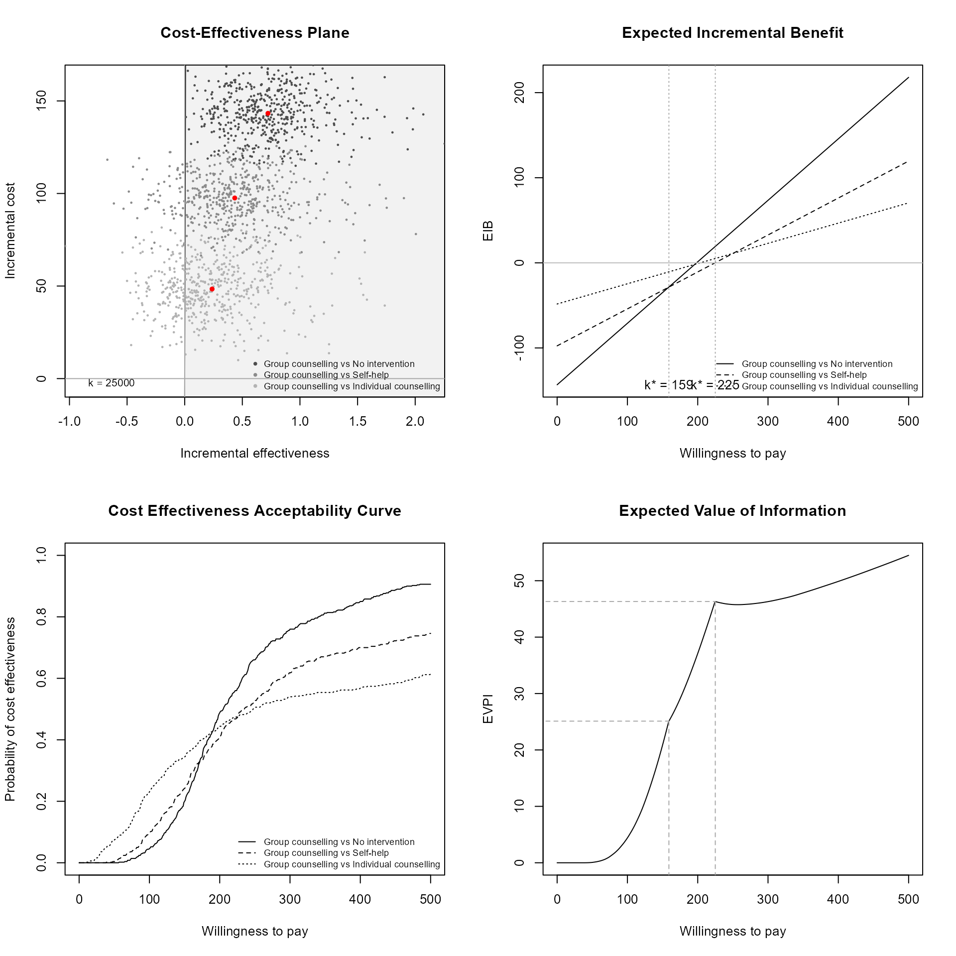
bcea_smoke <- bcea(eff, cost, ref = 4, interventions = treats, Kmax = 500)

We can easily create a grid of the most common plots

library(ggplot2)
library(purrr)

plot(bcea_smoke)

Individual plots can be plotting using their own functions.

ceplane.plot(bcea_smoke, comparison = 2, wtp = 250)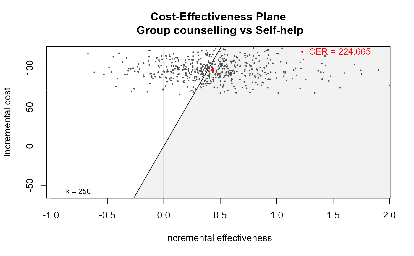


eib.plot(bcea_smoke)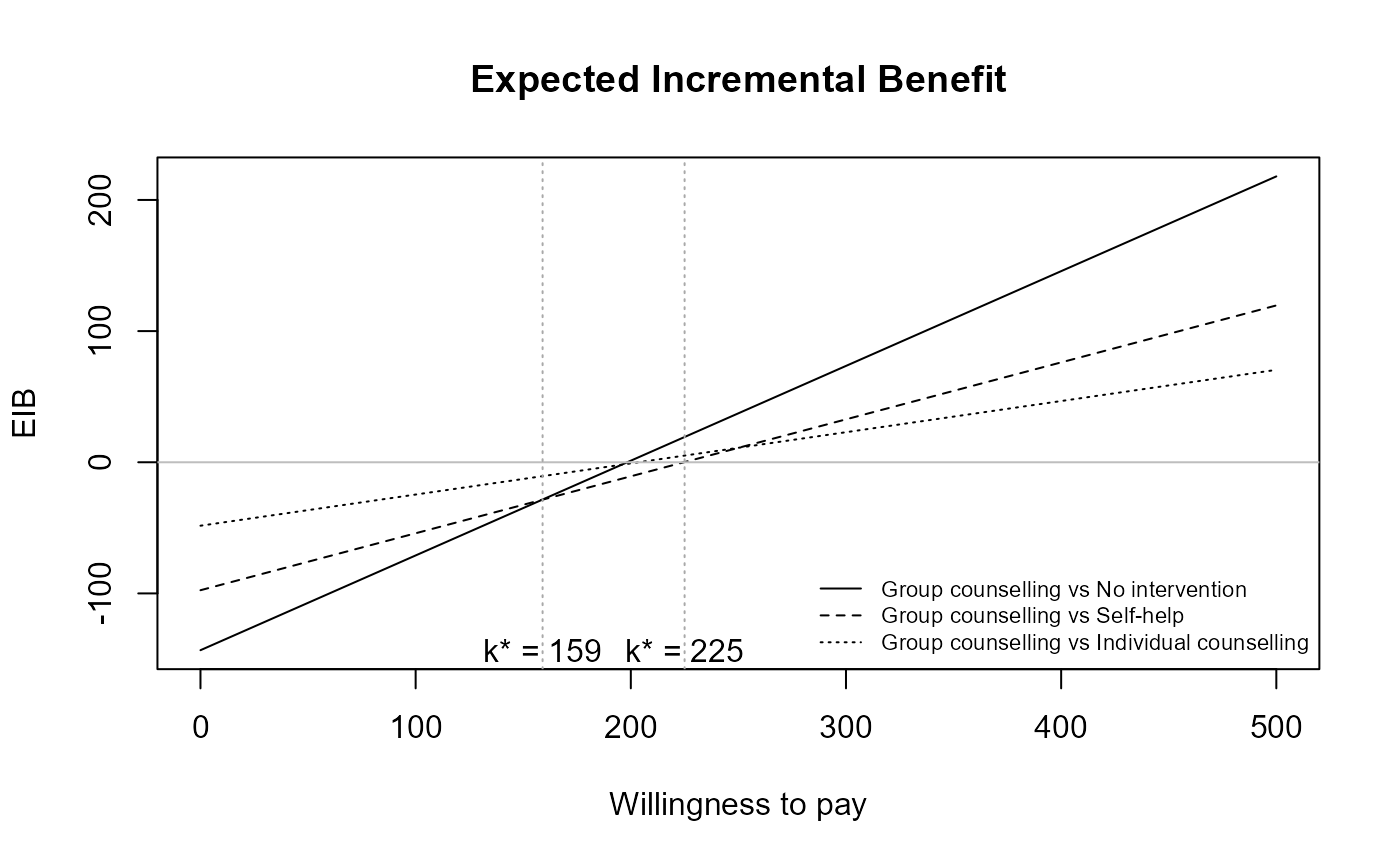


contour(bcea_smoke)


ceac.plot(bcea_smoke)


ib.plot(bcea_smoke)
#> NB: k (wtp) is defined in the interval [0 - 500]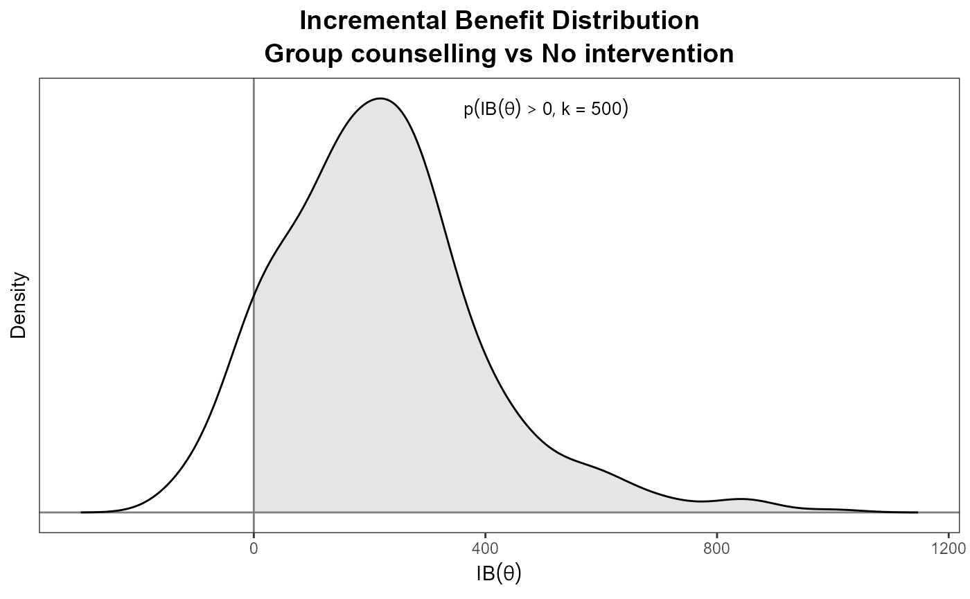

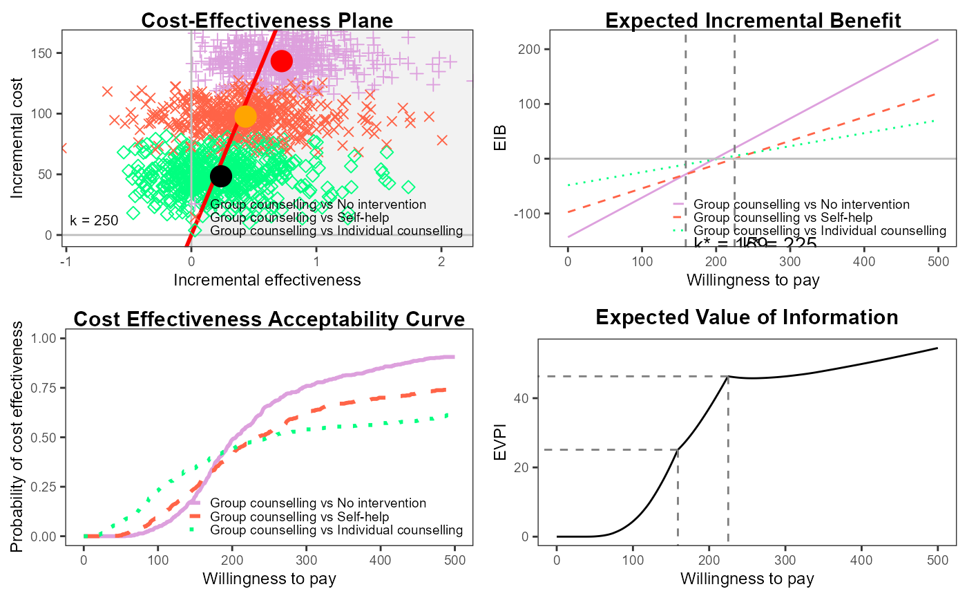
More on this in the other vignettes but you can change the default plotting style, such as follows.

plot(bcea_smoke,
     graph = "ggplot2",
     wtp = 250,
     line = list(color = "red", size = 1),
     point = list(color = c("plum", "tomato", "springgreen"), shape = 3:5, size = 2),
     icer = list(color = c("red", "orange", "black"), size = 5))