Expected Incremental Benefit Plot

Introduction

The intention of this vignette is to show how to plot different styles of expected incremental benefit (EIB) plots using the BCEA package.

Two interventions only

This is the simplest case, usually an alternative intervention (\(i=1\)) versus status-quo (\(i=0\)).

The plot is based on the incremental benefit as a function of the willingness to pay \(k\).

\[ IB(\theta) = k \Delta_e - \Delta_c \]

Using the set of \(S\) posterior samples, the EIB is approximated by

\[ \frac{1}{S} \sum_s^S IB(\theta_s) \]

where \(\theta_s\) is the realised configuration of the parameters \(\theta\) in correspondence of the \(s\)-th simulation.

R code

To calculate these in BCEA we use the bcea() function.

data(Vaccine)

he <-
  bcea(eff, cost,                  
       ref = 2,                
       interventions = treats, 
       Kmax = 50000,
       plot = FALSE)

The default EIB plot gives a single diagonal line using base R.

eib.plot(he)

The vertical line represents the break-even value corresponding to \(k^*\) indicating that above that threshold the alternative treatment is more cost-effective than the status-quo.

\[ k^* = \min\{ k : \mbox{EIB} > 0 \} \]

This will be at the point the curve crosses the x-axis.

The plot defaults to base R plotting. Type of plot can be set explicitly using the graph argument.

eib.plot(he, graph = "base")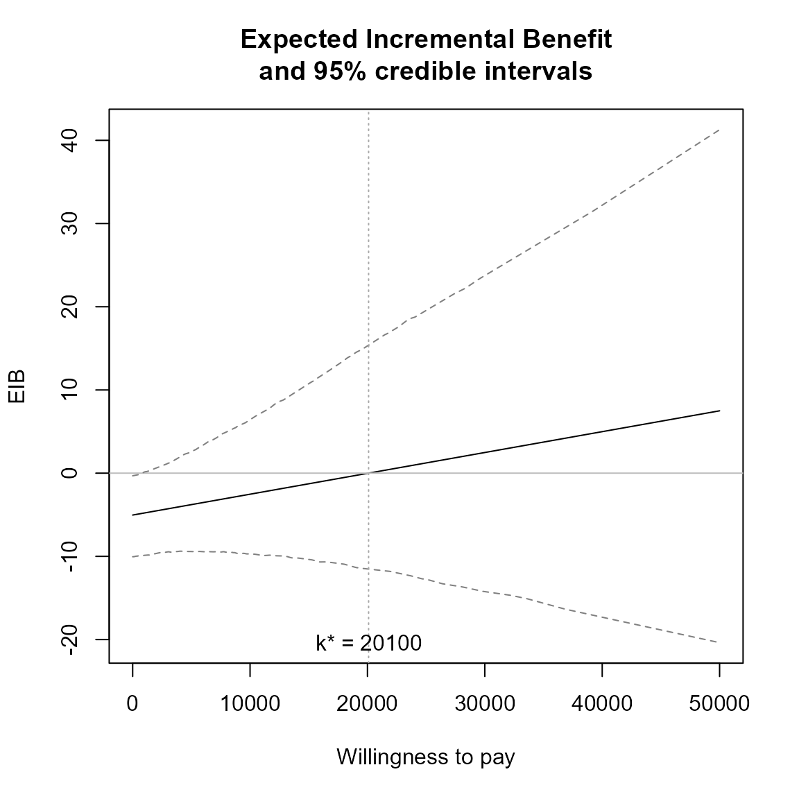

eib.plot(he, graph = "ggplot2")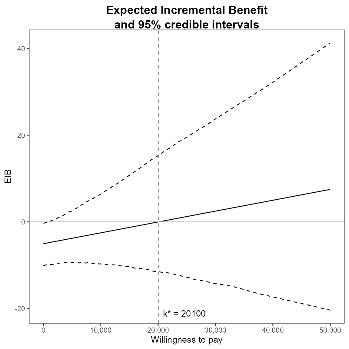

# ceac.plot(he, graph = "plotly")

Other plotting arguments can be specified such as title, line colours and theme.

eib.plot(he,
         graph = "ggplot2",
         main = "my title",
         line = list(color = "green"),
         theme = theme_dark())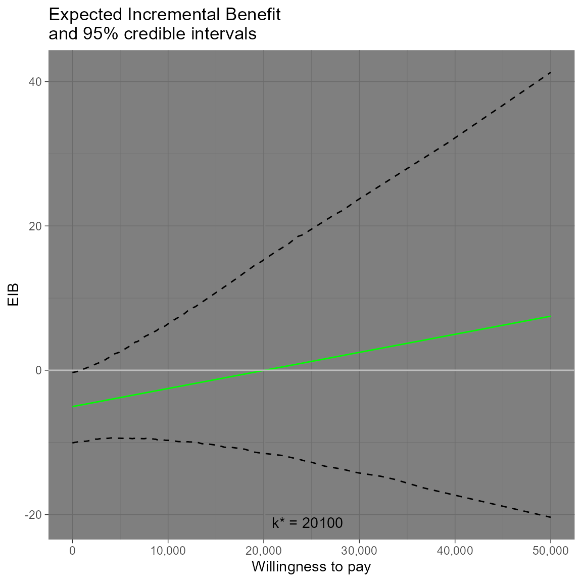

Credible interval can also be plotted using the plot.cri logical argument.

eib.plot(he, plot.cri = FALSE)

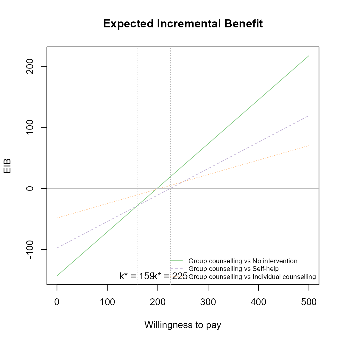
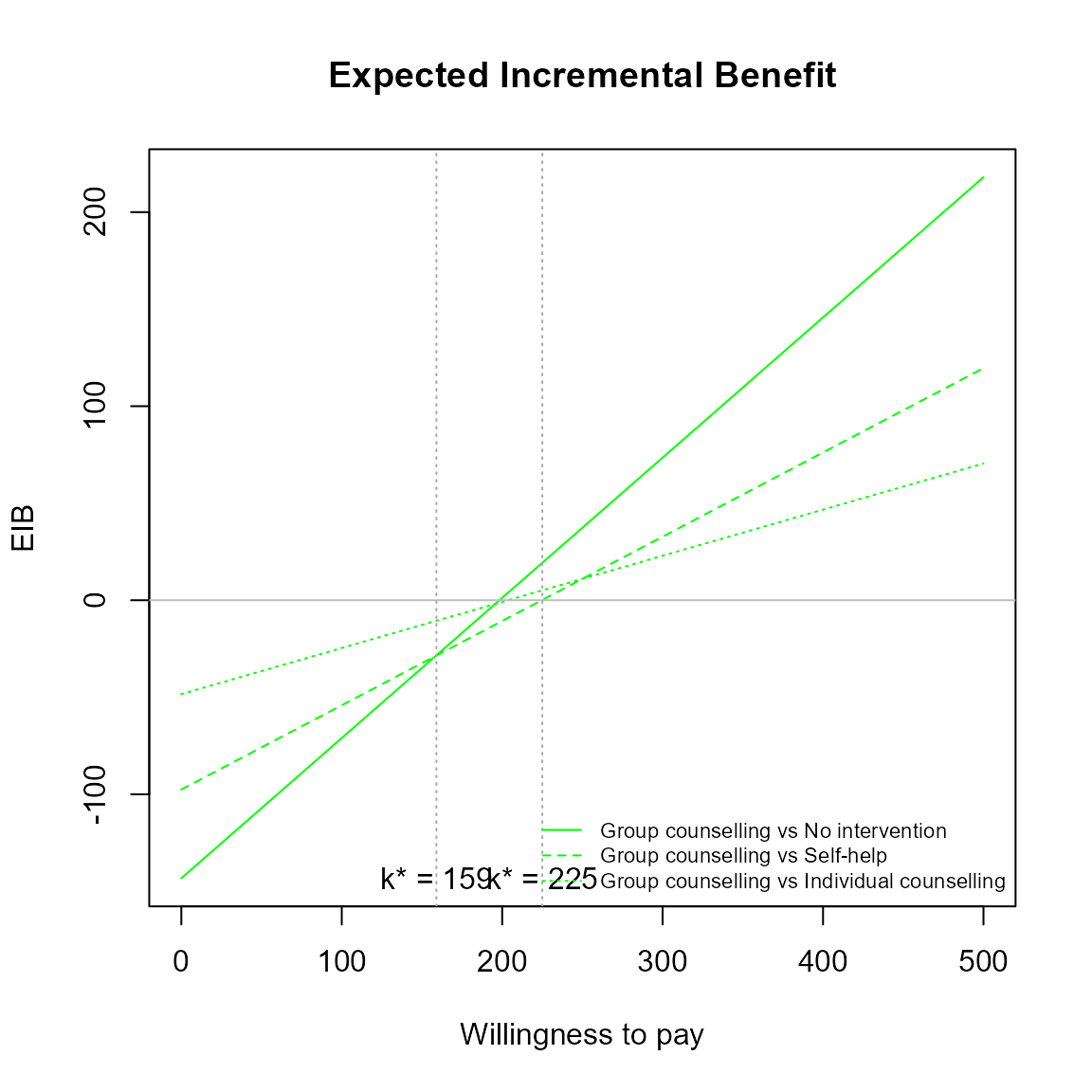
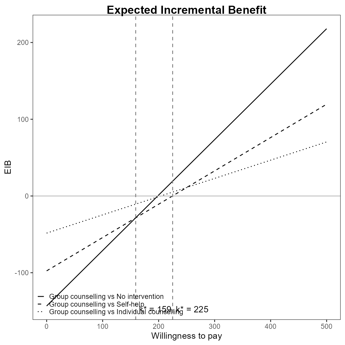
Multiple interventions

This situation is when there are more than two interventions to consider. Incremental values can be obtained either always against a fixed reference intervention, such as status quo, or for all comparisons simultaneously.

The curves are for pair-wise comparisons against a status-quo and the vertical lines and k* annotation is for simultaneous comparisons.

Without loss of generality, if we assume status quo intervention \(i=0\), then we wish to calculate

\[ \frac{1}{S} \sum_s^S IB(\theta^{i0}_s) \;\; \mbox{for each} \; i \]

The break-even points represent no preference between the two best interventions at \(k\).

\[ k^*_i = \min\{ k : \mbox{EIB}(\theta^i) > \mbox{EIB}(\theta^j) \} \]

Only the right-most of these will be where the curves cross the x-axis.

R code

This is the default plot for eib.plot() so we simply follow the same steps as above with the new data set.

data(Smoking)

treats <- c("No intervention", "Self-help",
            "Individual counselling", "Group counselling")
he <- bcea(eff, cost, ref = 4, interventions = treats, Kmax = 500)

eib.plot(he)

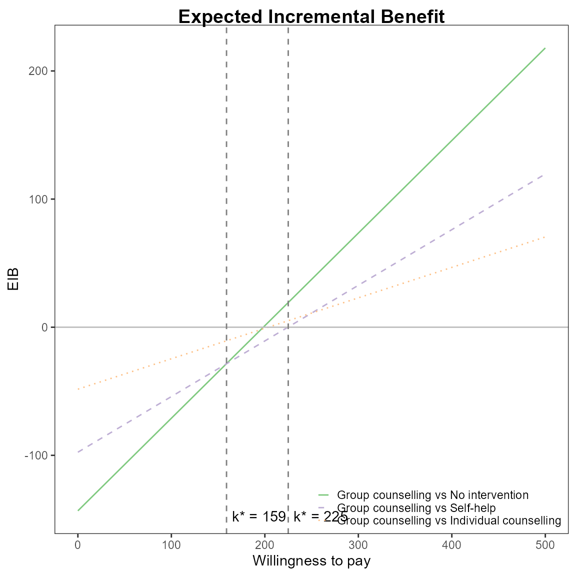
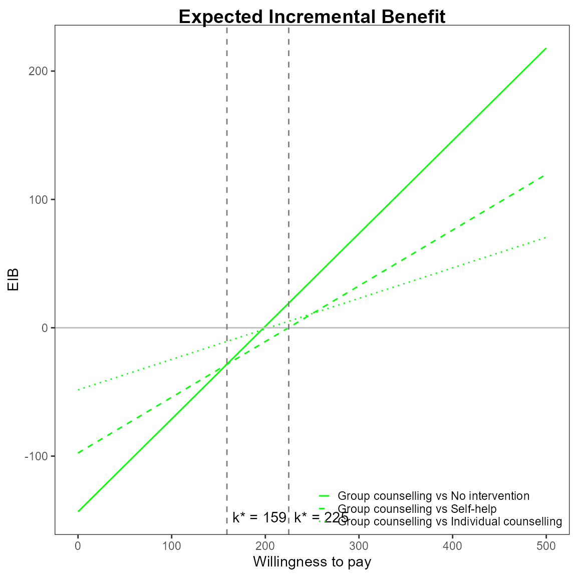
For example, we can change the main title and the EIB line colours to green.

eib.plot(he,
         graph = "base",
         main = "my title",
         line = list(color = "green"))

eib.plot(he,
         graph = "ggplot2",
         main = "my title",
         line = list(color = "green"))

Credible interval can also be plotted as before. This isn’t recommended in this case since its hard to understand with so many lines.

eib.plot(he, plot.cri = TRUE)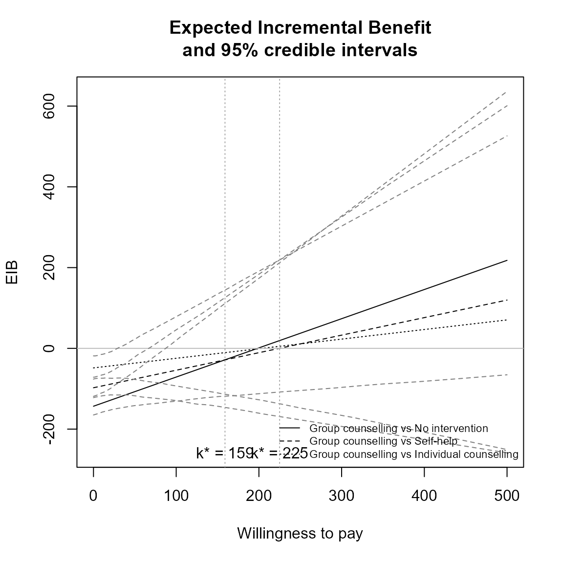

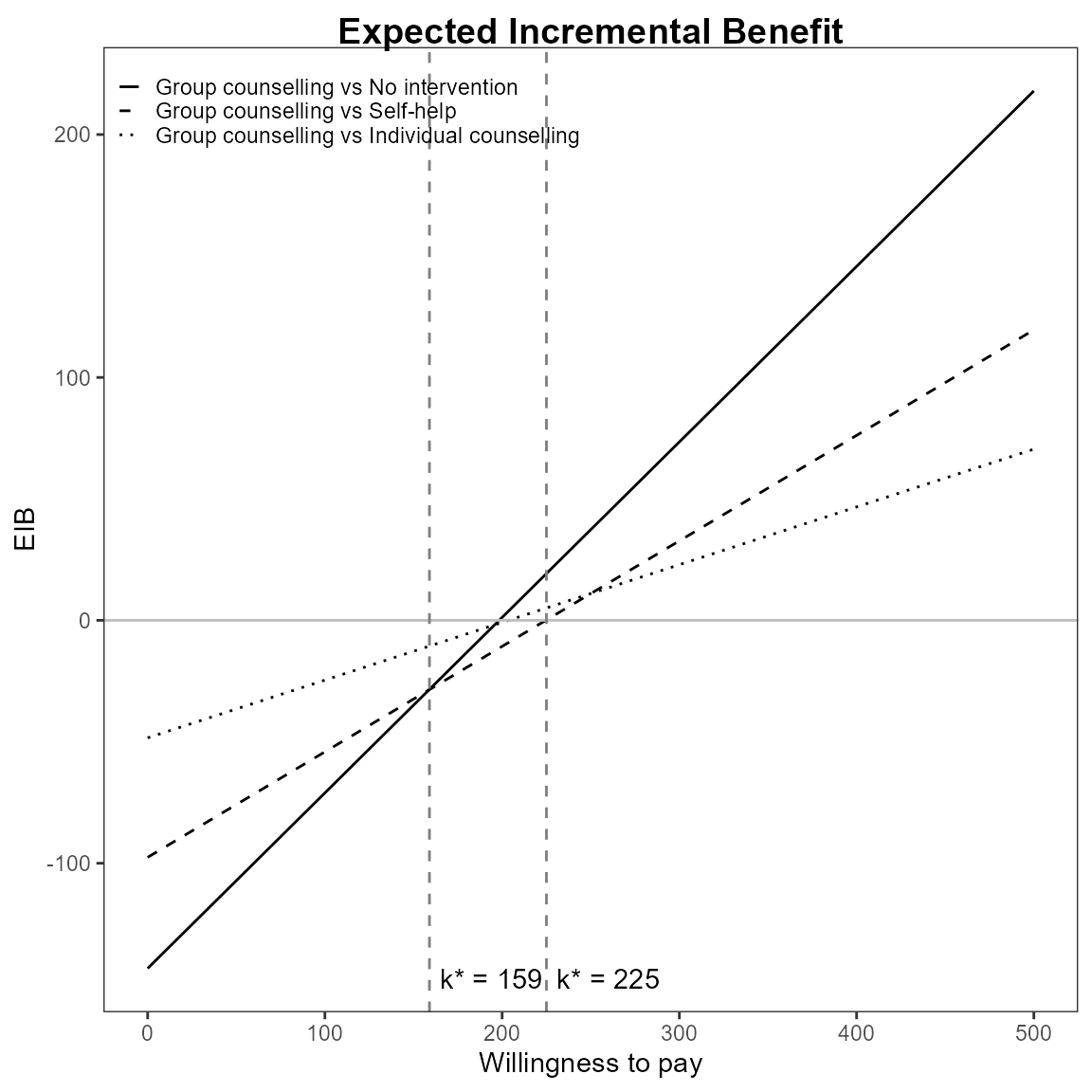
Repositioning the legend.

For base R,

eib.plot(he, pos = FALSE) # bottom right

eib.plot(he, pos = c(0, 0))

eib.plot(he, pos = c(0, 1))

eib.plot(he, pos = c(1, 0))

eib.plot(he, pos = c(1, 1))

For ggplot2,

##TODO:
eib.plot(he, graph = "ggplot2", pos = c(0, 0))

eib.plot(he, graph = "ggplot2", pos = c(0, 1))

eib.plot(he, graph = "ggplot2", pos = c(1, 0))

eib.plot(he, graph = "ggplot2", pos = c(1, 1))

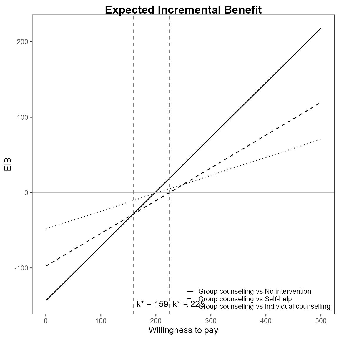
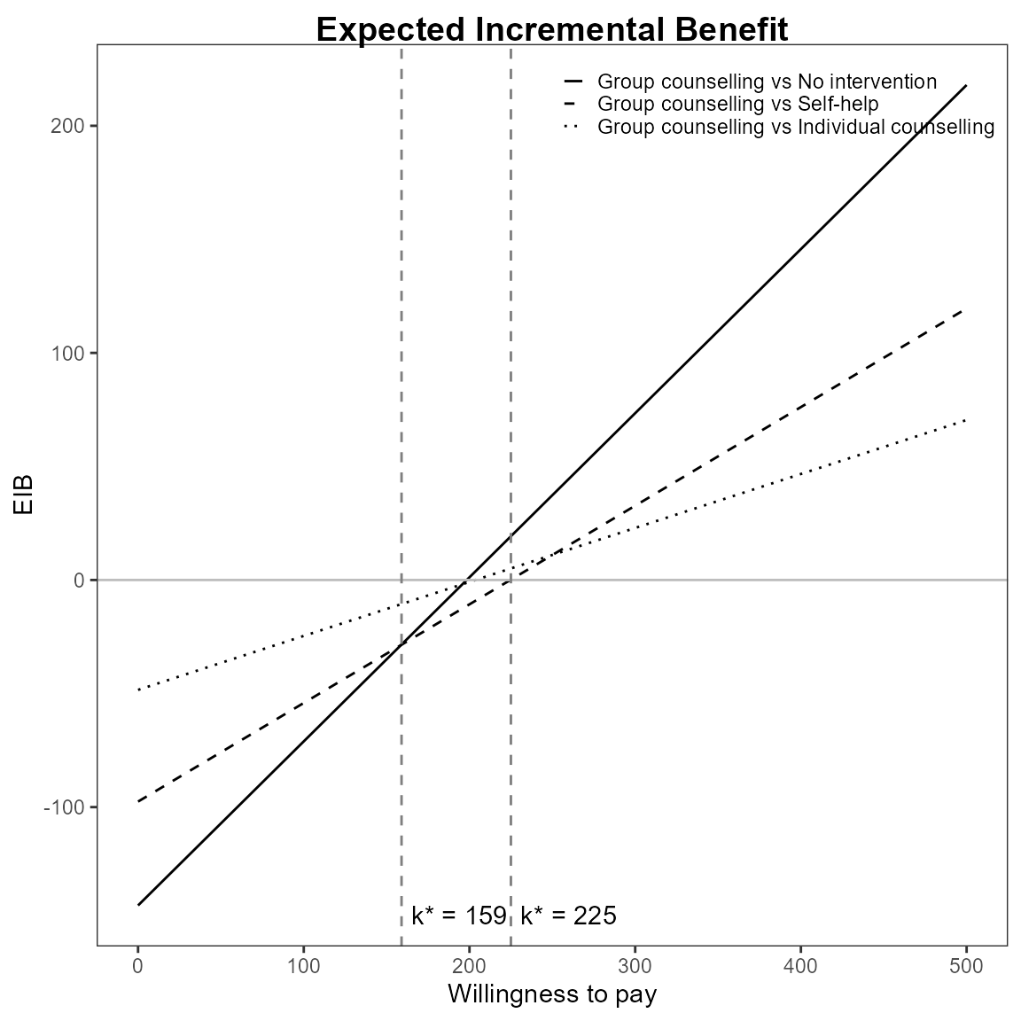
Define colour palette for different colour for each EIB line.

mypalette <- RColorBrewer::brewer.pal(3, "Accent")

eib.plot(he,
         graph = "base",
         line = list(color = mypalette))

eib.plot(he,
         graph = "ggplot2",
         line = list(color = mypalette))