Cost-effectiveness plane

##TODO…

Introduction

The intention of this vignette is to show how to plot different styles of cost-effectiveness acceptability curves using the BCEA package.

R code

To calculate these in BCEA we use the bcea() function.

data("Vaccine")

he <- bcea(eff, cost)
#> No reference selected. Defaulting to first intervention.

The plot defaults to base R plotting. Type of plot can be set explicitly using the graph argument.

ceplane.plot(he, graph = "base")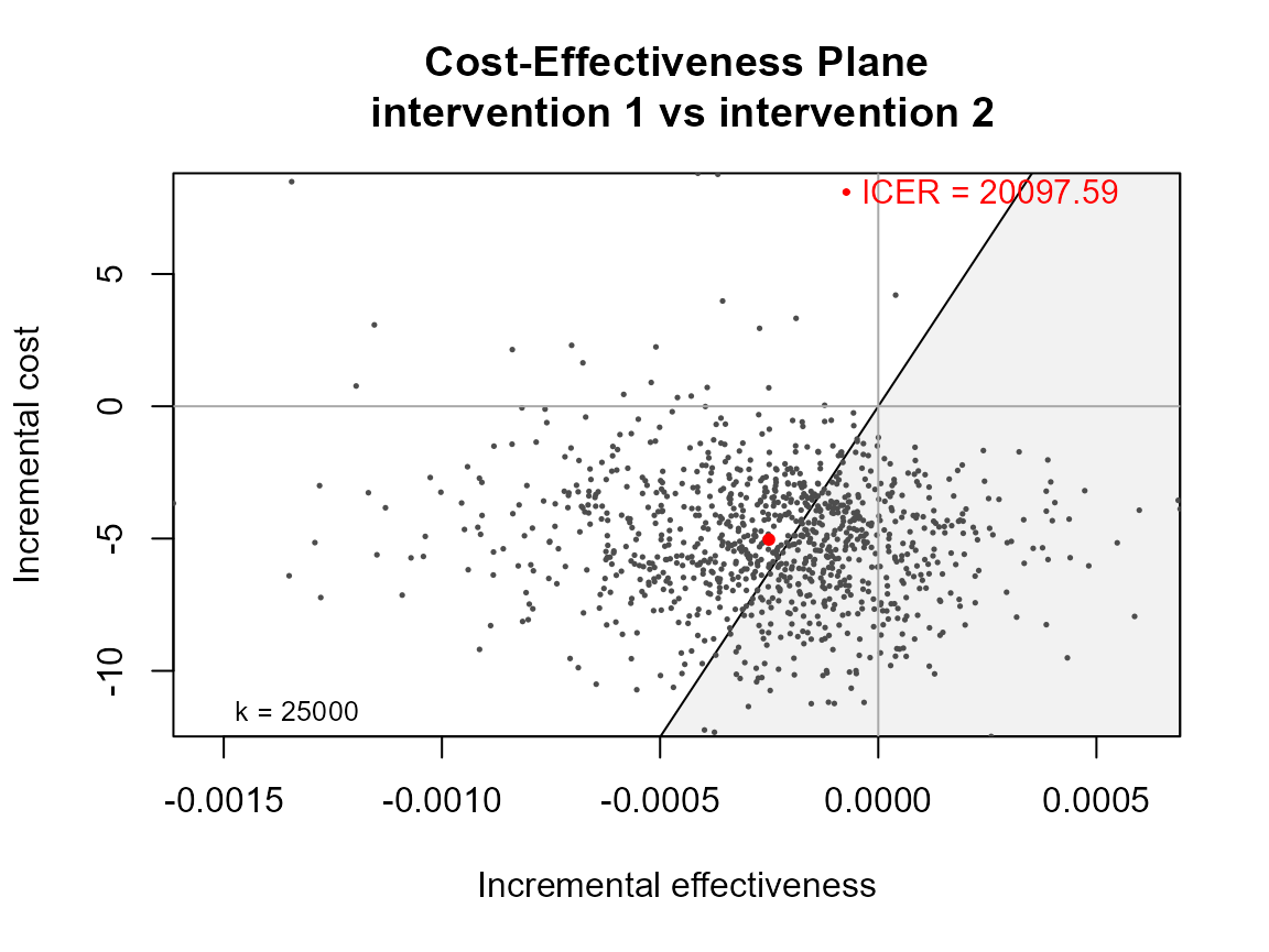

ceplane.plot(he, graph = "ggplot2")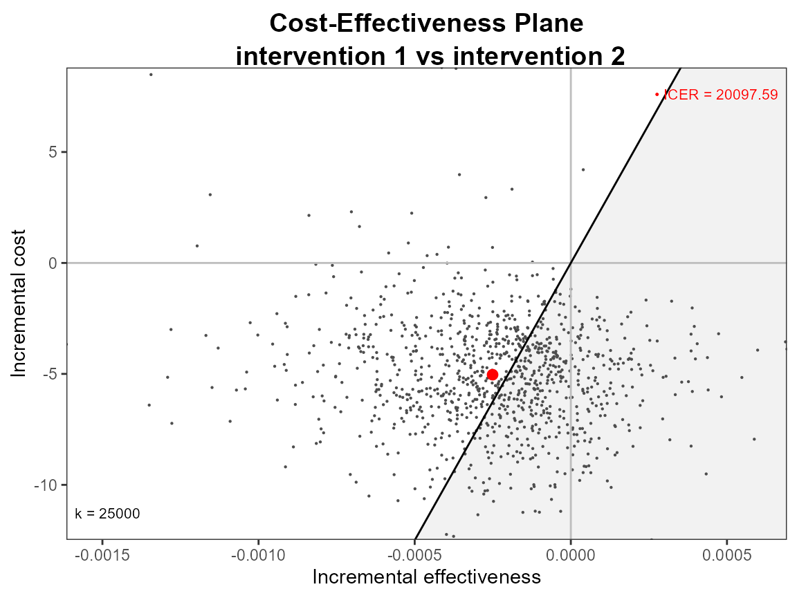

# ceac.plot(he, graph = "plotly")

Other plotting arguments can be specified such as title, line colours and theme.

ceplane.plot(he,
             graph = "ggplot2",
             title = "my title",
             line = list(color = "green", size = 3),
             point = list(color = "blue", shape = 10, size = 5),
             icer = list(color = "orange", size = 5),
             area = list(fill = "grey"),
             theme = theme_linedraw())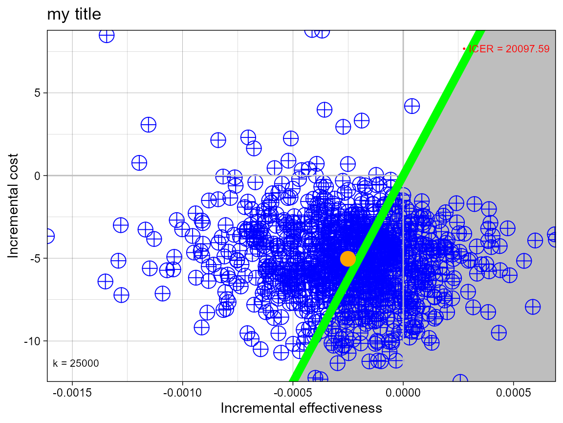

If you only what the mean point then you can suppress the sample points by passing size NA.

ceplane.plot(he,
             graph = "ggplot2",
             point = list(size = NA),
             icer = list(size = 5))
#> Warning: Removed 1000 rows containing missing values (`geom_point()`).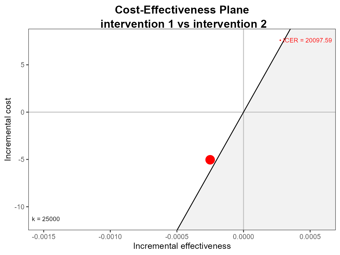

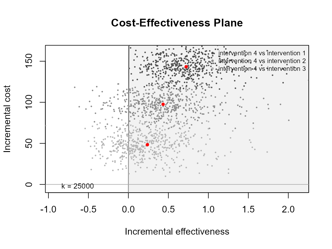
Multiple interventions

This situation is when there are more than two interventions to consider.

R code

data("Smoking")

he <- bcea(eff, cost, ref = 4)
# str(he)

ceplane.plot(he)

ceplane.plot(he, graph = "ggplot2")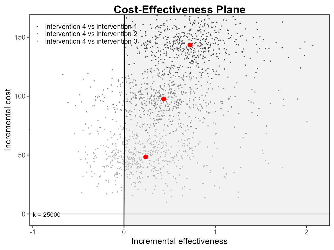

ceplane.plot(he,
             graph = "ggplot2",
             title = "my title",
             line = list(color = "red", size = 1),
             point = list(color = c("plum", "tomato", "springgreen"), shape = 3:5, size = 2),
             icer = list(color = c("red", "orange", "black"), size = 5))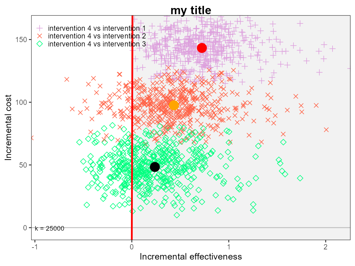

Reposition legend.

ceplane.plot(he, pos = FALSE) # bottom right

ceplane.plot(he, pos = c(0, 0))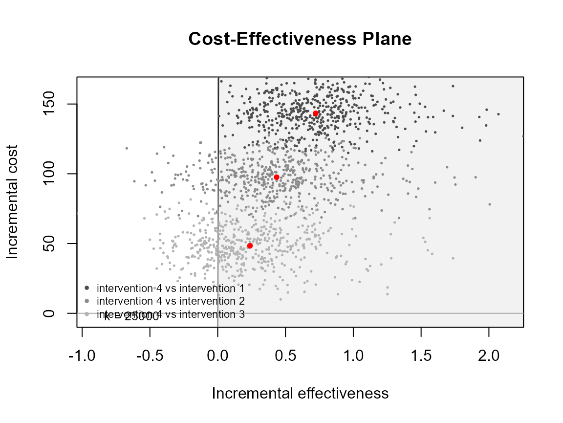

ceplane.plot(he, pos = c(0, 1))

ceplane.plot(he, pos = c(1, 0))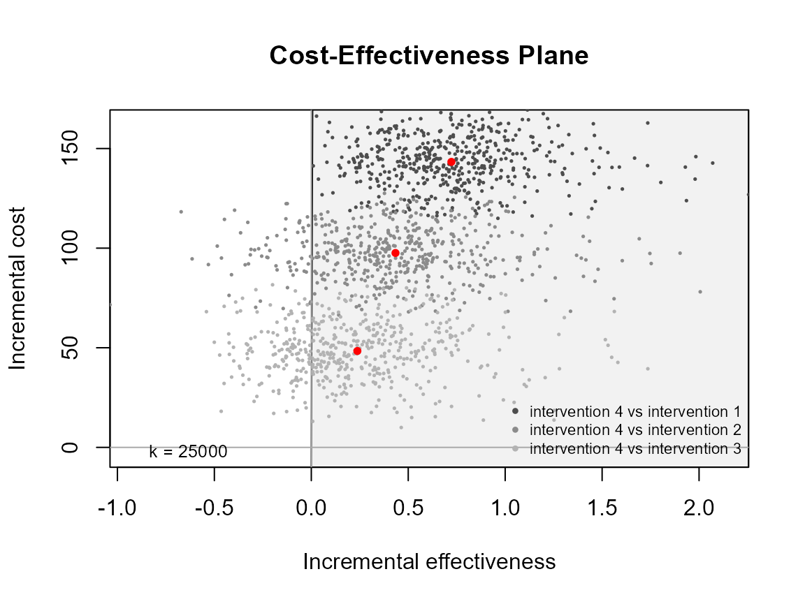

ceplane.plot(he, pos = c(1, 1))