Specialised CE-plane Contour Plot

Produces a scatterplot of the cost-effectiveness plane, with a contour-plot of the bivariate density of the differentials of cost (y-axis) and effectiveness (x-axis). Also adds the sustainability area (i.e. below the selected value of the willingness-to-pay threshold).

Usage

# S3 method for bcea
contour2(
  he,
  comparison = NULL,
  wtp = 25000,
  graph = c("base", "ggplot2"),
  pos = c(0, 1),
  ...
)

contour2(he, ...)

Arguments

he: A bcea object containing the results of the Bayesian modelling and the economic evaluation.
comparison: The comparison being plotted. Default to NULL If graph_type="ggplot2" the default value will choose all the possible comparisons. Any subset of the possible comparisons can be selected (e.g., comparison=c(1,3)).
wtp: The selected value of the willingness-to-pay. Default is 25000.
graph: A string used to select the graphical engine to use for plotting. Should (partial-)match the three options "base", "ggplot2" or "plotly". Default value is "base". Not all plotting functions have a "plotly" implementation yet.
pos: Parameter to set the position of the legend (only relevant for multiple interventions, ie more than 2 interventions being compared). Can be given in form of a string (bottom|top)(right|left) for base graphics and bottom|top|left|right for ggplot2. It can be a two-elements vector, which specifies the relative position on the x and y axis respectively, or alternatively it can be in form of a logical variable, with FALSE indicating to use the default position and TRUE to place it on the bottom of the plot.
...: Arguments to be passed to ceplane.plot(). See the relative manual page for more details.

Value

contour: A ggplot item containing the requested plot. Returned only if graph_type="ggplot2".

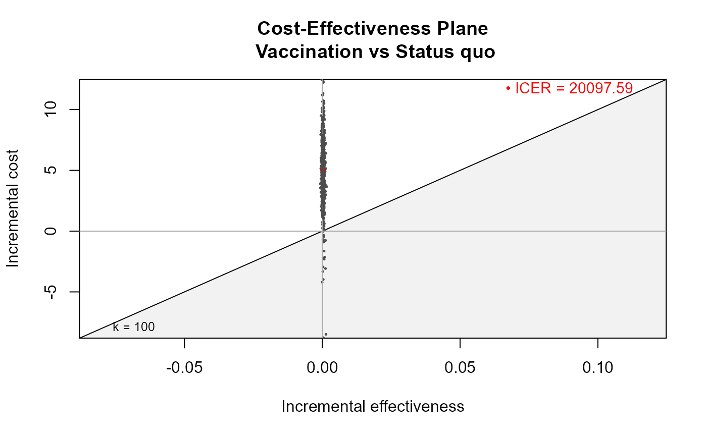
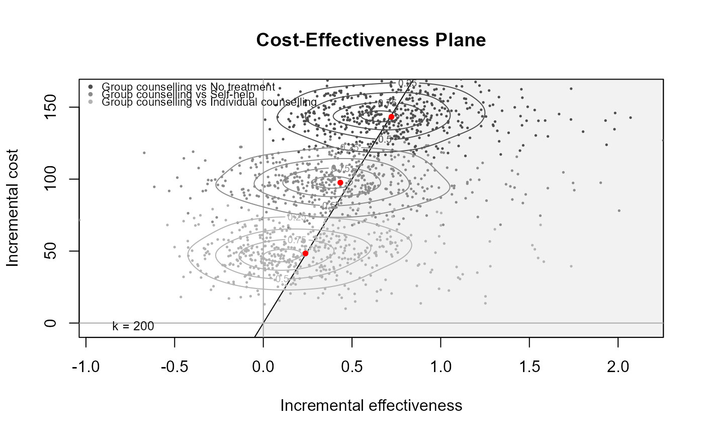
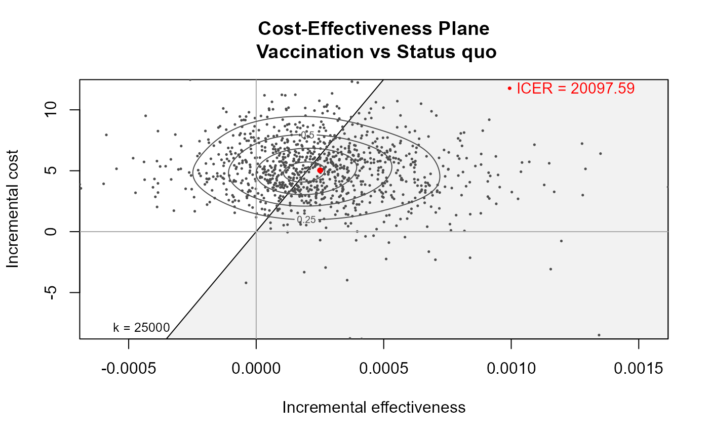
Plots the cost-effectiveness plane with a scatterplot of all the simulated values from the (posterior) bivariate distribution of (\(\Delta_e, \Delta_c\)), the differentials of effectiveness and costs; superimposes a contour of the distribution and prints the value of the ICER, together with the sustainability area.

References

Baio G, Dawid aP (2011). “Probabilistic sensitivity analysis in health economics.” Stat. Methods Med. Res., 1--20. ISSN 1477-0334, doi:10.1177/0962280211419832 , https://pubmed.ncbi.nlm.nih.gov/21930515/.

Baio G (2013). Bayesian Methods in Health Economics. CRC.

Author

Gianluca Baio, Andrea Berardi

Examples

## create the bcea object m for the smoking cessation example
data(Smoking)
m <- bcea(eff, cost, ref = 4, interventions = treats, Kmax = 500)

## produce the plot
contour2(m,
         wtp = 200,
         graph_type = "base")

# \donttest{
## or use ggplot2 to plot multiple comparisons
contour2(m,
         wtp = 200,
         ICER_size = 2,
         graph_type = "ggplot2")

# }

## vaccination example
data(Vaccine)
treats = c("Status quo", "Vaccination")
m <- bcea(eff, cost, ref = 2, interventions = treats, Kmax = 50000)
contour2(m)

contour2(m, wtp = 100)