Produces a plot the Cost-Effectiveness Acceptability Frontier (CEAF) against the willingness to pay threshold.
Usage
# S3 method for pairwise
ceaf.plot(mce, graph = c("base", "ggplot2"), ...)

ceaf.plot(mce, ...)
Arguments
- mce
The output of the call to the function
multi.ce()- graph
A string used to select the graphical engine to use for plotting. Should (partial-) match the two options
"base"or"ggplot2". Default value is"base".- ...
Additional arguments
References
Baio G, Dawid aP (2011). “Probabilistic sensitivity analysis in health economics.” Stat. Methods Med. Res., 1--20. ISSN 1477-0334, doi:10.1177/0962280211419832 , https://pubmed.ncbi.nlm.nih.gov/21930515/.
Baio G (2013). Bayesian Methods in Health Economics. CRC.
Examples
# See Baio G., Dawid A.P. (2011) for a detailed description of the
# Bayesian model and economic problem
# Load the processed results of the MCMC simulation model
data(Vaccine)
# Runs the health economic evaluation using BCEA
m <- bcea(
e=eff,
c=cost, # defines the variables of
# effectiveness and cost
ref=2, # selects the 2nd row of (e, c)
# as containing the reference intervention
interventions=treats, # defines the labels to be associated
# with each intervention
Kmax=50000, # maximum value possible for the willingness
# to pay threshold; implies that k is chosen
# in a grid from the interval (0, Kmax)
plot=FALSE # inhibits graphical output
)
# \donttest{
mce <- multi.ce(m) # uses the results of the economic analysis
# }
# \donttest{
ceaf.plot(mce) # plots the CEAF
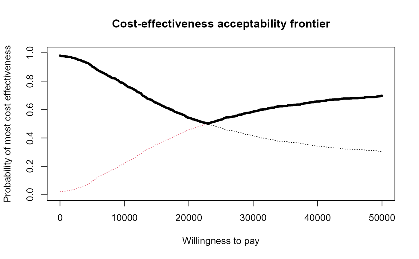 # }
# \donttest{
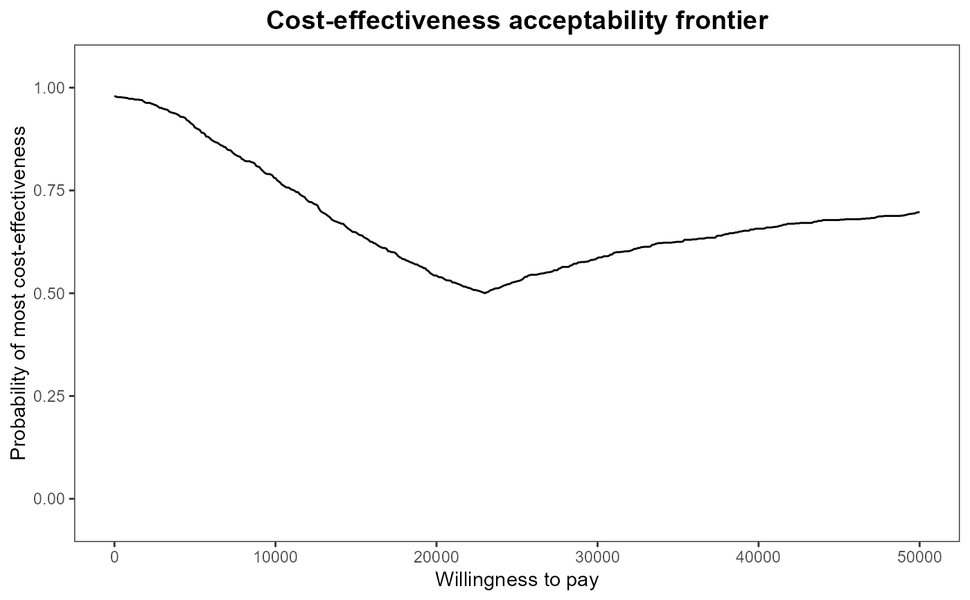
ceaf.plot(mce, graph = "g") # uses ggplot2
# }
# \donttest{
ceaf.plot(mce, graph = "g") # uses ggplot2
 # }
# \donttest{
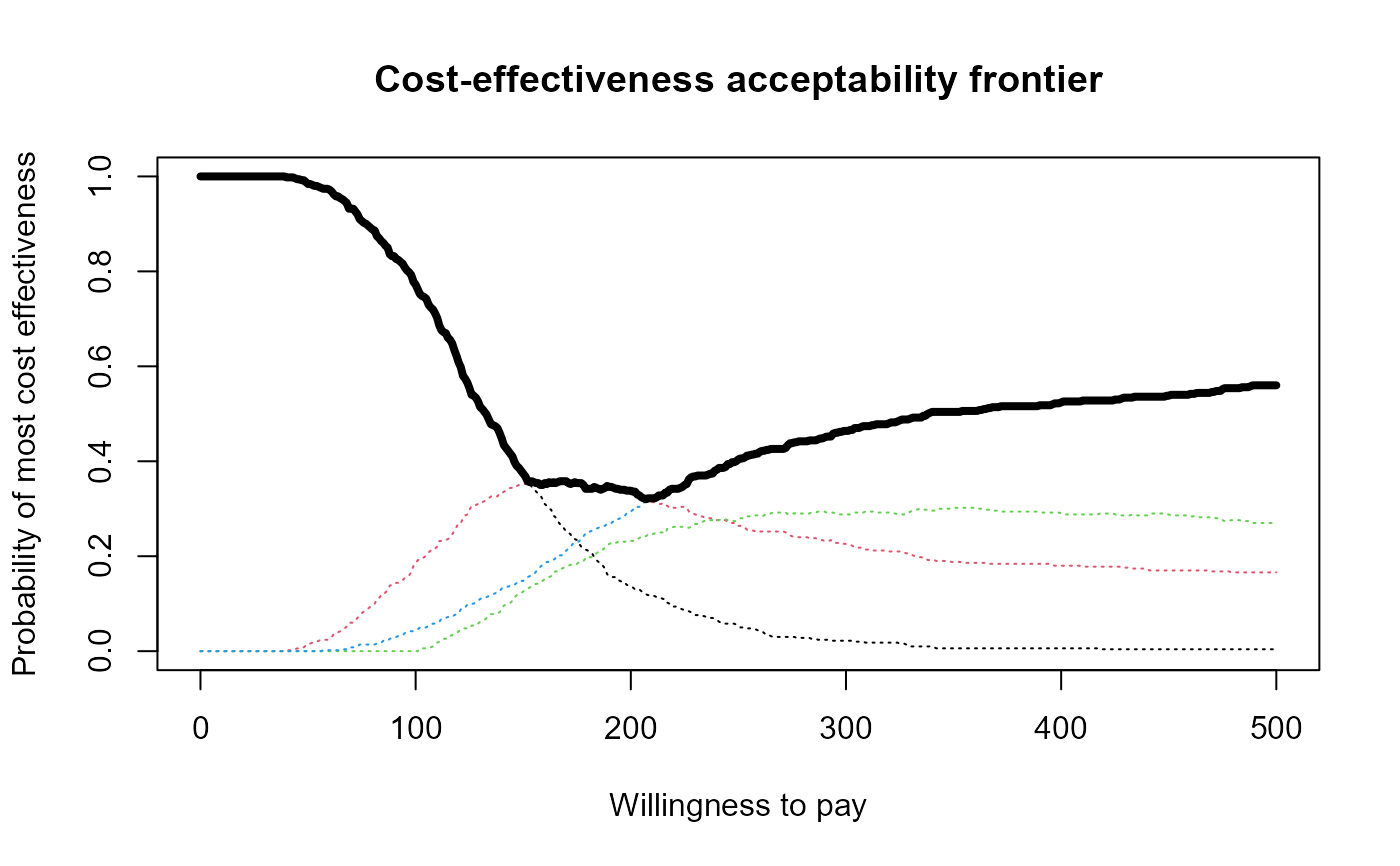
# Use the smoking cessation dataset
data(Smoking)
m <- bcea(eff, cost, ref = 4, intervention = treats, Kmax = 500, plot = FALSE)
mce <- multi.ce(m)
ceaf.plot(mce)
# }
# \donttest{
# Use the smoking cessation dataset
data(Smoking)
m <- bcea(eff, cost, ref = 4, intervention = treats, Kmax = 500, plot = FALSE)
mce <- multi.ce(m)
ceaf.plot(mce)
 # }
# }