Exercises: RMarkdown
Exercises: RMarkdown
In this practical we will introduce the basics of using RMarkdown and some of its features.
Introduction
R Markdown is a file format for making dynamic documents with R. An R Markdown document is written in markdown (an easy-to-write plain text format) and contains chunks of embedded R code.
An RMarkdown document is rendered by knitting the file.
The rmarkdown package will call the knitr package. knitr will run
each chunk of R code in the document and append the results of the code
to the document next to the code chunk. This workflow saves time and
facilitates reproducible reports.
Consider how authors typically include graphs (or tables, or numbers) in a report. The author makes the graph, saves it as a file, and then copy and pastes it into the final report. This process relies on manual labour. If the data changes, the author must repeat the entire process to update the graph.
In the R Markdown paradigm, each report contains the code it needs to make its own graphs, tables, numbers, etc. The author can automatically update the report by re-knitting.
Creating a R Markdown document
To create an R Markdown report, open a plain text file and save it with the extension .Rmd. You can open a plain text file in your scripts editor by clicking File > New File > Text File in the RStudio tool bar, or using the Wizard by selecting File > New File > R Markdown …
Rendering
To go from R Markdown to pdf or html you can click on the Knit icon
thats above the file in the scripts editor. A drop down menu will let
you select the type of output that you want. RStudio will show you a
preview of the new output and save the output file in your working
directory. You can manually render an R Markdown file with
rmarkdown::render().
Text formatting
Markdown is designed to be easy to read and easy to write. It is also very easy to learn.
Go to the drop down menu and select Help > Markdown Quck Reference. This will open a cheat sheet in the Help pane.
Code chunks
To run code inside an R Markdown document, you need to insert a chunk. There are three ways to do so:
-
The keyboard shortcut Cmd/Ctrl + Alt + I
-
The Insert button icon in the editor tool bar
-
By manually typing the chunk delimiters
{r} and.
Think of a chunk like a function. A chunk should be relatively self-contained, and focussed around a single task.
Chunk names
Chunks can be given an optional name: ```{r by-name}. This has three advantages:
-
You can more easily navigate to specific chunks using the drop-down code navigator in the bottom-left of the script editor:
-
Graphics produced by the chunks will have useful names that make them easier to use elsewhere. More on that in other important options.
-
You can set up networks of cached chunks to avoid re-performing expensive computations on every run.
Chunk options
Chunk output can be customised. A full list is here http://yihui.name/knitr/options/.
The most important set of options controls if your code block is executed and what results are inserted in the finished report:
-
eval = FALSEprevents code from being evaluated. (And obviously if the code is not run, no results will be generated). This is useful for displaying example code, or for disabling a large block of code without commenting each line. -
include = FALSEruns the code, but doesn’t show the code or results in the final document. Use this for setup code that you don’t want cluttering your report. -
echo = FALSEprevents code, but not the results from appearing in the finished file. Use this when writing reports aimed at people who don’t want to see the underlying R code. -
message = FALSEorwarning = FALSEprevents messages or warnings from appearing in the finished file. -
results = 'hide'hides printed output;fig.show = 'hide'hides plots. -
error = TRUEcauses the render to continue even if code returns an error. This is rarely something you’ll want to include in the final version of your report, but can be very useful if you need to debug exactly what is going on inside your .Rmd. It’s also useful if you’re teaching R and want to deliberately include an error. The default, error = FALSE causes knitting to fail if there is a single error in the document.
Tables in R Markdown
By default, R Markdown prints data frames and matrices as you’d see them
in the console. If you prefer that data be displayed with additional
formatting you can use the knitr::kable function. For even deeper
customisation, consider the xtable, stargazer, pander, tables,
and ascii packages
Inline code
To embed R code in a line of text, surround the code with a pair of back ticks and the letter r, like this.
`r ICER is 200/0.5`
knitr will replace the inline code with its result in your final document (inline code is always replaced by its result). The result will appear as if it were part of the original text
YAML header
A YAML header to control how rmarkdown renders your .Rmd file. A YAML header is a section of key: value pairs surrounded by — marks.
The output: value determines what type of output to convert the file
into when you call rmarkdown::render().
output: recognizes the following values:
html_document, which will create HTML output (default)pdf_document, which will create PDF outputword_document, which will create Word output
If you use the RStudio IDE knit button to render your file, the selection you make in the gui will override the output: setting.
Putting it all together in an example report
-
Create a new R Markdown document with main sections with headings Introduction, Data, Methods, Results and Conclusions.
-
Include some subheadings like Model Fitting and Recommendations, say.
-
In the Conclusions make numbered list of the main findings.
-
Include a link to the Briggs papers on which the original cost-effectiveness analysis is based i.e. An Introduction to Markov Modelling for Economic Evaluation, Andrew Briggs and Mark Sculpher
-
Change the date of the document so that it will always be today’s date using the following
date: "`r format(Sys.time(), '%d %B, %Y')`"
Pick a date format that you prefer
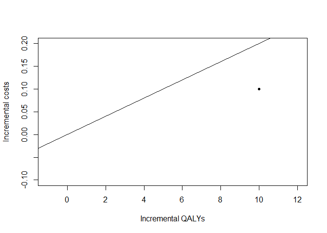
- Include the plot created with the following code
plot(10, 0.1,
     xlab = "Incremental QALYs",
     ylab = "Incremental costs",
     xlim = c(-1, 12),
     ylim = c(-0.1, 0.2),
     pch = 20)
abline(a = 0, b = 0.02)
-
Resize this plot using the chunk options
-
Add a caption using
fig.cap -
Create a table that shows the cost and QALYs for two interventions and their incremental values and ICER. Here something to start with. What do the colons do?
intervention | cost | QALY | delta c | delta QALY | ICER
-------------|-----:|-----:|---------|------------|-----
- Now create the same table but do this programmatically. That is
create a data frame with the entries and then use
knitr::kableto convert to markdown.
Here’s an example template to get you started using data.frame:
data.frame(intervention = c("drug a", "drug b"))|>
knitr::kable()
-
What would be an advantage of using
tibble::tribblehere? -
Some times you just want the R code without any of the extra text. The
purlfunction in thekintrpackage takes an input file, extracts the R code in it according to a list of patterns, evaluates the code and writes the output in another file. Usepurlwith your R Markdown document. -
Sometimes when a document becomes large it is easier to split it up in to smaller document and then combine these in a top level file. This is possible in R Markdown using children chunks. Simply use the argument
childassigned to the name of theRmdfile and this will be inserted in to the document in place of this chunk.
{r child = 'mychilddoc.Rmd'}
Create a Methods block and a Results child chunk for your current document.
This all just the tip of the iceberg. To find out more check out the R Markdown book here https://bookdown.org/yihui/rmarkdown/.